The program HAXIS was develop by Zhanyong Guo, Elfi Kraka, and Dieter Cremer for the purpose of:
- providing a global and a local description of helix distortions via a global and a local definition of the helix axis
The axis is derived from a coarse-grained (a residue is represented by the Cα atom as suitable anchor point) and spline-fitted backbone line of the helix provided by the APSA method. At each anchor point of the helix the Frenet frame of the backbone line is calculated, which leads directly to a vector presentation of the helix axis: The conformation of each residue contributes to the winding of the helix and thereby to the axis direction. In the case of ideal helices, all local axis directions coincide and lead to one overall axis vector. In the case of a real helix, irregularities in the winding of the helix are reflected by different axis directions per residue and therefore a zigzagging axis line. For the determination of the global shape of a helix the axis line is smoothened by a polynomial fit of third order and its curving and twisting calculated. HAXIS can also use a 5th order polynomial fit for describing kinked helices or a 2nd order fit when comparing with methods based on a circular fit.
The majority of all short helices (2 to 5 turns) is curved and twisted as is reflected by the distribution of average curvature and torsion. The shorter a helix is, the more likely is a larger distortion from its regular shape. Utilizing the calculated curvature radius C, the variation ΔC, and the ratio ηc = ΔC / Cav, helices are classified as being linear (18%), moderately curved (54%), or strongly curved (28%). Long helices are preferentially linear and seem to be more resistant to distortions.
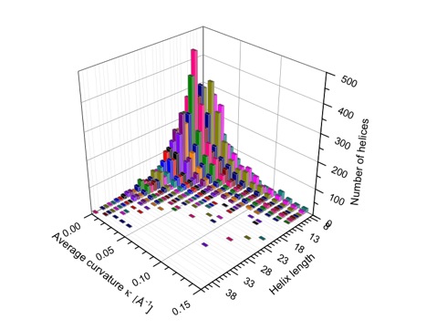
Average curvature in Å-1 of protein helices in dependence of the helix length (i.e. number of residues) given as general distribution in form of a 3D bar diagram (color is used to distinguish between helices of length m and m+1.
Both with the global and the local description, the kinking of a helix can be quantitatively assessed. Very reliable is the analysis of the local curvature of the helix axis. At the position of a helix kink, a characteristic peak pattern (quadruple configuration of peaks) is found, which leads to an easy identification of kinking and strongly curved helices. On the average, 5.8% of protein helices are kinked. For more details, click here.
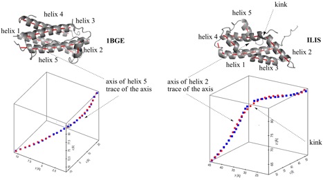
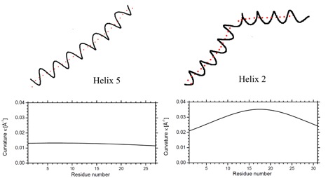
Helix n of protein 1BGE n = 5; left) and protein 1LIS n = 2; right). A.) Top: Ribon presentation. The calculated axes are given for all helices by red tubes. Bottom: Third order (1BGE, helix 5) and fifth order (1LIS, helix 2) polynomial fit (red points) for the calculated axis points (blue points). The perspective drawing provides an impression of the bending and twisting of the helix axis, which is not correctly comprehended when using a projection of a helix axis into a plane. B.) Top: Helix n and trace of its fitted axis (red dots). Bottom: Calculated curvature of the axis of helix n (based on a third or fifth order polynomial fit of the helix axis) as a function of the helix length (counting the first residue of helix n as residue 1).
The characteristic curvature changes are used to identify the start and exit of a helix. Alternatively the rise parameters ai can be used for this purpose or for the differentiation between helices and coils.
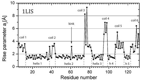
Representation of the rise parameter ai for protein 1LIS as a function of the residue number. Five helices (h) and six coils can be identified (dashed lines give start and end of helix). Residue 61 in helix 2 gives the position of a kink.
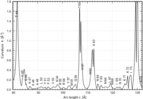
Curvature diagram of the spline-fitted axis of helix n in protein 1BGE (above, n = 5) and 1LIS (below, n = 2). Bending as well as kinking involves always several residues: A155 to A160 in 1BGE and T60 to A63 in 1LIS. Note that at the ends of the helix the transition to a coil or turn causes an increase in curvature.
HAXIS has several advantages compared to other approaches previously published. The majority of these methods is based on the assumption of a regular bending of the helix axis as described by a circle fitting, which leads to a simplified (sometimes false) description of axis bending. Twisting of the helix axis can no longer be described in this way because bending as given by a second order polynomial exclusively takes place in one plane. HAXIS corrects the simplified helix presentations and quantifies axis torsion.
The HAXIS method is the basis for a rapid classification and comparison of calculated and measured helix structures and in this way can be used in connection with a coarse-grained description of proteins. For more details, click here.
Descriptions of the Diagrams Generated by the HAXIS Program
P1) Presentation of the rise parameter ai The rise parameter ai (i is the residue counter) measures the difference in the positions of residues i to i+1 after projection onto the helix axis. It differs for alpha (ca. 1.5 Å), 3_10 (ca. 2 Å), and pi-helices (ca. 1 Å) as described in the HAXIS publication (Paper 342). Formally one can calculate also an axis for ß-strands, loops, coils, and turns by applying the same approach. Only in the latter cases, the rise parameters are significantly larger than 2 Å and irregular. In the figure P1 the rise parameters are given for all residues of the proteins. Those of the helix can easily be identified: A23 – N35. Systematic study of the rise parameters for ß-strands, loops, etc. can lead to new a description of these secondary structural units.
P2) Presentation of the curvature k as a function of the arc length s of the helix axis (given for each helix in the protein) The curvature of the helix axis (calculated by HAXIS and fitted by a fifth order polynomial; see HAXIS publication (Paper 342).) is given as a function of the arc length s and the positions of the anchor-points (Cα) of the residues forming the helix are given by dots and the appropriate residue symbol. As an example, the helix from A23 to N35 is shown. The helix axis is strongly bent toward its center (E27 – F30) as indicated by 4 curvature peaks. It is almost linear toward its end (small curvature peaks).
P3) Presentation of the spline-fitted axis of the entire protein As mentioned for P1, a local axis can be calculated not only for helices but also for ß-strands, coils, loops, or turns. These local axes are connected in the 3-dimensional perspective representation (in x,y,z-space) with the help of cubic spline-fits to a smooth line representing no longer the backbone line of the protein but the axis line of the secondary structural units. The only helix (A23 – N35) is easily recognized because its axis corresponds to the regularly bent (almost horizontal) line in the upper part of the diagram.
P4) Presentation of the position of the helix axis with regard to the protein backbone line (given for each helix in the protein) A simple backbone line is generated by connecting the Cα anchor points of the residues. The helix axis is indicated by red dots, which correspond to the positions of the helix residues projected onto the helix axis.
P5) Enlargement of P4 showing just the helix (given for each helix in the protein) Backbone line and helix axis (given by red dots) are shown exclusively. This plot is generated in the same way as P4, however only the helix in question is shown.
HAXIS Output Example
HAXIS Main Program & Description
            ############################################################################
            HAXIS main program
            Protein helix axis analysis
            by Daniel Guo, Elfi Kraka, Dieter Cremer, CATCO, SMU
            version 0.0.1 (test purpose)
            ----------------------------------------------------------------------

            Requirement:	Python. Linux environment preferred. Other platform untested.
            Dependency:	numpy
                DSSP, if use DSSP secondary structure assignment

            Usage:	Run command from Bash (Linux) or Terminal.app (Mac) in the current(working) directory with the path to the input files as argument. For example, run the following  				 		python /path/to/haxis/haxis.py /path/to/input_file

            The program works on PCs (windows) and Macs (terminal application). However, in order to run the DSSP program on a Mac environment the user needs to install the boost library and use a special DSSP version. Details are described in a folder, which is included in the program package to be downloaded.

            ############################################################################

            Please note, 3 test examples and the corresponding output files are collected in the sub folder “test” of the haxis program folder

            ############################################################################

            # Input file  The input files consists of four  lines of settings at the beginning that follow  certain format:
            # Line 1: /path/to/pdb.	This is the full path where pdb files are located
            # Line 2: option:  	two digit options, 1st digit: helix definition (0-3), see below. Default value is 0		  			   2nd digit: switch for extra analysis by using HAXIS helix definition. Either 0 or 1 (1 turns it on). Default value is 0.
            # Line 3: output folder. Default is current folder. When use current folder, leave this line empty.
            # Line 4: /path/to/dssp:	path to dssp executable if 1st digit is set to 2 (leave blank if 1st digit option above is others)

            # Helix definitions for 1st digit option (0-3):
            0	Identification of a helix by HAXIS. Currently, HAXIS looks for segments showing regular geometry parameters: rise parameter a, radius, arc length and curvature peak (of fitted axis curve), and angle of neighboring local axis directions. Where the regular region ends are the start/ends of helix.
            1	use helix definition that is provided by the pdb file
            2	use DSSP assignment. DSSP executable required
            3	custom defined helix definition. A text file with helix definition is required. The file name should be the same as the regular output file with “.hx” as extension. E.g. 2GB1A.hx

            # line5…n: pdb_name  chain_id  model_id
            Beginning from line 5 is a list of protein structures to be analyzd. One structure per line.
             where  chain_id: is the chain identifier of a single polymer chain in a pdb file (x-ray structure)
                model_id: is the model identifier of a single model in the ensemble of NMR structures
            # Example: The given path to the pdb files is "/media/sf_vms/hh/pdb/". The 2 digit option is "21" for helix definition 2 and switching dssp on. The output folder is default (empty line indicates current folder). The path to the dssp executable is "../dssp". There is one helix each line, begins with the starting residue # and ends with the ending residue # separated by Tab.

            test31
            ############################################################################
            #line 1: full path where pdb files are located,
            #line 2: option switch xx. First x is helix definition (0-2), default is 0; second x is extra analysis by using HAXIS internal helix definition, default value 0 is off, set to 1 to turn on.
            #line 3: output folder. Default is current folder. When use current folder, leave this line empty.
            #line 4: path to dssp executable if option switch 1 in line2 is 2. Otherwise leave this line empty.
            /Users/Desktop/haxisv001a8/pdb/
            31
            /Users/Desktop/haxisv001a8/test/test31
            ../dssp
            2GB1	A
            1BGE	A
            1LIS	A
            ############################################################################

            View the output of the example here:
            http://smu.edu/catco/downloads/haxis_output.pdf


            ############################################################################
            # Output files:
            1	.haxis	main output file

            1.1	input line
            1.2	alignment of residue ID and helix definition
            1.3	C_ alpha coordinates and Frenet coordinates of C_alpha
            Residue # | residue id | x,y,z coordinates of CA | arc length | curvature | torsion
            1.4	Frenet vectors
            T: tangent vector, N: principal normal, B: binormal vector of spline curve connecting C_alpha positions. Each vector is defined by x,y,z coordinates of its end point.
            1.5	Axis
            x,y,z coordinates of the anchor points of the traces of generalized local axes of the entire protein backbone
            1.6	Rise a_i per residue
            Helix rise parameter a_i per residue
            1.7	Helices
            Beginning and ending of each helix
            1.8	Helix axis traces
            x,y,z coordinates of each anchor point of the trace of the local helix axis (projection of C_alpha on to axis)
            1.9	Polynomial fit of the helix axis: coefficients a_0  ->  a_n
            2nd order polynomial fit
            3rd order polynomial fit
            5th order polynomial fit
            1.10	Curvature kappa and torsion tau of the curved helix axis presented by a polynomial fit of 2nd, 3rd of 5th order.

            1.11	helix classification and global geometry parameters
            Helix  (beginning and ending residue #)
            Shape:   LC: weakly curved, HC: highly curved, L: linear
            Regularity: R: regular, IR: irregular, SI: strongly irregular
            C_av: average radius of curvature
            C_max: maximum radius of curvature
            delta_C:   Variation of radius of curvature
            delta_C/C_av
            k_av: average curvature
            k_max: maximum curvature
            delta_k:  Variation of radius of curvature
            delta_k/k_av
            Type: conventional type L: linear, C: curved, K: kinked
            1.12	kink (based on irregularity of rise)
            Helix beginning and ending residue | kink position | rise value | variation of rise over average rise of given helix segment
            1.13	kink (based on curvature quartet (i.e. 4 curvature peaks) of axis)
            pdb id | kink position | Helix beginning and ending residue | kink region (residues involved in the k quartet) | peak curvature k value of kink quartet | corresponding rise value

            If extra analysis switch is turned on, section 1.7-1.13 repeat for second analysis.

            2	.gp gnuplot script for a graphical representation of the rise parameter a, the curvature of the helix axis, the spline fitted local axis, the local axis for the entire protein and the individual helices.
            Use the following command to generate figure in .ps format:
            gnuplot filename.gp

            File 3 and 4 are data files required to generate figures in file 2:

            3	.axsp	arc length, curvature and torsion of fitted spline over generalized global axis of entire protein.
            Format:
            Segmental arc length | accumulated arc length | curvature | torsion | x,y,z coordinates of axis traces | curvature at the point corresponding to the projection of CA on the axis (anchor point of spline fit) | residue ID | residue number

            4	.dca	.dca includes coordinates of protein backbone and local axis points.

            5	if extra analysis is turned on, extra files: protein_name2.gp , .dca files for the extra analysis.


            ############################################################################
             #Generating Gnuplot figures

            From command line:
            cd Directory/To/Output/Files
            gnuplot "filename.gp"

            Inside gnuplot:
            load "filename.gp"


            ############################################################################
            #Extra notes

            The pdb files with protein structure coordinates are available from Protein Data Bank at:
            http://www.rcsb.org/

            DSSP is an independent way of defining protein secondary structures. The program is available at:
            http://swift.cmbi.ru.nl/gv/dssp/
            HAXIS includes the dssp routine which uses the DSSP helix definition.

            END
            ############################################################################
